


Next: 7 Channel couplings
Up: Methods of Direct Reaction
Previous: 5 Distorted Wave Born
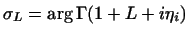
6 Partial-wave expansions
The total wave function is expanded in partial waves using a coupling
order such as
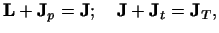 |
|
|
(30) |
which may be defined by writing
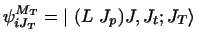 |
|
|
(31) |
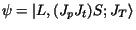
where
Jp
= projectile spin,
Jt
= target spin,
L
= orbital partial wave, and
JT
= total system angular momentum.
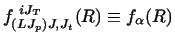
The set
{i, (L Jp )J, Jt ; JT }
will be abbreviated by the single variable  .
Thus, in each partition the partial wave expansion of the
wave function is
.
Thus, in each partition the partial wave expansion of the
wave function is
| |
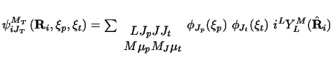 |
|
|
| |
 |
|
(32) |
here  and
and  are the internal coordinates of the projectile and target, and
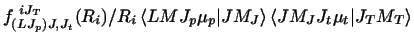
 |
|
|
(33) |
are the radial wave functions.
The (optional) iL factors are included to simplify the spherical Bessel expansion of the
incoming plane wave.
The wave function  could also have been defined using the `channel
spin' representation
could also have been defined using the `channel
spin' representation
 ,
which is symmetric upon projectile
,
which is symmetric upon projectile  target interchange except for
a phase factor
(-1)S - Jp - Jt.
The coupled partial-wave equations
are of the form
target interchange except for
a phase factor
(-1)S - Jp - Jt.
The coupled partial-wave equations
are of the form
where the partial-wave kinetic energy operator is
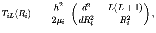 |
|
|
(35) |
Ui (Ri) is the diagonal optical potential
with nuclear and Coulomb components,
and Rm is a radius limit larger than the ranges of
Ui (Ri) and of the coupling terms.
The
 are the local
coupling interactions of multipolarity
are the local
coupling interactions of multipolarity  , and the
 are the non-local couplings between mass
partitions that arise from particle transfers.
The equations (34) are in their most common form;
they become more complicated when
non-orthogonalities are included by the method of section 8.1.
For incoming channel
are the non-local couplings between mass
partitions that arise from particle transfers.
The equations (34) are in their most common form;
they become more complicated when
non-orthogonalities are included by the method of section 8.1.
For incoming channel  , the solutions
 satisfy the boundary conditions when Ri > Rm of
![$\displaystyle f_\alpha {(R_i)}=
{i \over 2} \left [ \delta_{\alpha\alpha_0 }
H^...
...i}} ( k_i R_i )
- S_{\alpha\alpha_0 }
H^{(+)}_{L {\eta_i}} ( k_i R_i )
\right ]$](img117.gif) |
|
|
(36) |
where
 and
and
 are the Coulomb functions with incoming and outgoing boundary conditions
respectively, and
are the Coulomb functions with incoming and outgoing boundary conditions
respectively, and
 |
|
|
(37) |
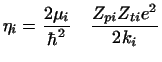
is the Sommerfeld parameter for the Coulomb wave functions.
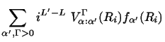
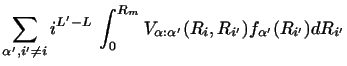
In terms of the S-matrix elements
 ,
and for coupling order of Eq. (30), the scattering
amplitudes for transitions to projectile & target m-states of m, M
to m', M' are
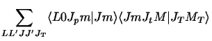
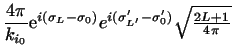
,
and for coupling order of Eq. (30), the scattering
amplitudes for transitions to projectile & target m-states of m, M
to m', M' are
where
 |
|
|
(39) |
are the Coulomb phase shifts and the Coulomb amplitude Fc is
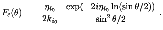 |
|
|
(40) |
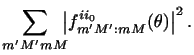
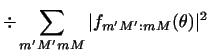
The corresponding differential cross section is
The spherical tensor analysing powers Tkq
describe how the outgoing
cross section depends on the incoming
polarisation state of the projectile.
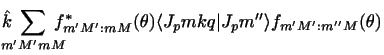
If the spherical tensor  is an operator with matrix elements
we have
Next: 7 Channel couplings
Up: Methods of Direct Reaction
Previous: 5 Distorted Wave Born
Prof Ian Thompson
2006-02-08


![$\displaystyle \left ( {i \over 2} \right )
\left [ \delta_{\alpha',\alpha} - S^{J_T}_{\alpha'\alpha} \right ]
~ Y_{L'}^{m' +M' -m-M}(\theta,0)$](img126.gif)