Next: 3 Model Schrödinger Equation
Up: Methods of Direct Reaction
Previous: 1 Direct Reaction Model
Subsections
Because the model space in direct reaction theory is not the whole
physical range, we need to define a division of
the full Hilbert space by means of projection operators. Following
Feshbach[7] we define P as the projection operator onto
the model space, including the entrance channels,
and Q as projecting on to the remaining space.
Such operators must obey P2=P, Q2=Q, PQ=QP=0 and P+Q=I,
where I is the identity operator. With these operators we divide
the physical wave function  of the system as
 where
where
 and
and
 . The
. The  component,
includes the elastic channel and just those channels `directly' related to it
that we choose to include in our direct reaction model.
The contains the same reaction channels as the
model wave function
component,
includes the elastic channel and just those channels `directly' related to it
that we choose to include in our direct reaction model.
The contains the same reaction channels as the
model wave function
 ,
but the wave functions are not identical since the model Hamiltonian
is obtained by some energy-averaging procedure to be discussed below.
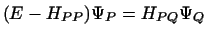
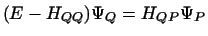
The physical Hamiltonian H governs the full wave function
at energy E by the Schrödinger equation
,
but the wave functions are not identical since the model Hamiltonian
is obtained by some energy-averaging procedure to be discussed below.
The physical Hamiltonian H governs the full wave function
at energy E by the Schrödinger equation  . This equation
is now separated into two coupled equations for and
. This equation
is now separated into two coupled equations for and  :
:
 |
|
|
(2) |
 |
|
|
(3) |
where
 ,
,
 and so on.
The Eq. (2) has an incoming wave boundary condition in the elastic
channel, and there are outgoing waves in all other channels of this
and Eq. (3) too. We may therefore formally solve Eq. (3)
as
and so on.
The Eq. (2) has an incoming wave boundary condition in the elastic
channel, and there are outgoing waves in all other channels of this
and Eq. (3) too. We may therefore formally solve Eq. (3)
as
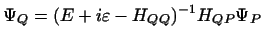 |
|
|
(4) |
and substitute this into Eq. (2) to obtain a formally exact
uncoupled equation for :
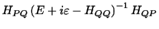
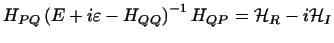
The Feshbach procedure therefore gives an effective Hamiltonian  for the
direct-reaction model space
for the
direct-reaction model space  :
:
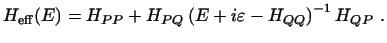 |
|
|
(5) |
This is an exact expression, and describes precisely the effect on the model
space all variations and resonances (for example) in the eliminated space.
The effective Hamiltonian however, is non-local and energy-dependent even
when the potential interactions in H are local and energy-independent.
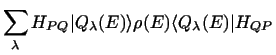
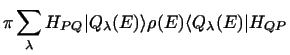
The contributions of distinct compound-nucleus state to the effective
Hamiltonian may be seen by expanding over a complete set of such states:
where  distinguishes among degenerate states. Then the
second term on the r.h.s of Eq. (5) becomes
distinguishes among degenerate states. Then the
second term on the r.h.s of Eq. (5) becomes
| |
|
 |
|
| |
= |
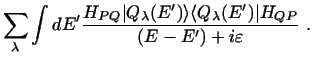 |
(6) |
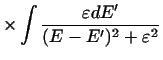
This term, from coupling to the Q channels, has
Hermitian and anti-Hermitian parts,
 |
|
|
(7) |
where
with  the density of states of HQQ at energy E.
The anti-Hermitian part
the density of states of HQQ at energy E.
The anti-Hermitian part  is positive definite, and
arises because the compound-nucleus channels act, asymmetrically,
only to remove flux from the the model-space channels that are in .
is positive definite, and
arises because the compound-nucleus channels act, asymmetrically,
only to remove flux from the the model-space channels that are in .
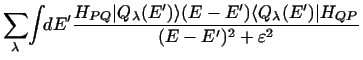
2.2 Energy Averaging
In direct reaction calculations, the precise compound nuclear resonances
are not needed in all their fluctuations, but only the average effect of these
and similar channels. This is most easily accomplished by averaging
 over small energy intervals, giving
 as
as
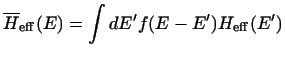 |
|
|
(11) |
where f(E-E') is some distribution function of unit integral and width
of the order  .
If is significantly larger than the average spacing of the
compound nucleus levels (
.
If is significantly larger than the average spacing of the
compound nucleus levels (
 ), then
the resulting
), then
the resulting
 has Hermitian and anti-Hermitian
components that vary rather slowly with energy E.
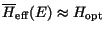
In order to formulate an Optical Model, we further assume that the
energy-averaged effective Hamiltonian
can
be approximated by a local potential that depends only on
the coordinate degrees of freedom that are explicitly treated in the model
wave function. That is, we approximate
has Hermitian and anti-Hermitian
components that vary rather slowly with energy E.
In order to formulate an Optical Model, we further assume that the
energy-averaged effective Hamiltonian
can
be approximated by a local potential that depends only on
the coordinate degrees of freedom that are explicitly treated in the model
wave function. That is, we approximate
 , which depends only
on the collective and/or single-particle degrees of freedom that
distinguish the particular N nuclei eigenstates
, which depends only
on the collective and/or single-particle degrees of freedom that
distinguish the particular N nuclei eigenstates  and
and
 .
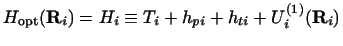
If the model space contains only the elastic channel (N=1),
we thereby reduce the effective Hamiltonian to contain a
local optical potential
.
If the model space contains only the elastic channel (N=1),
we thereby reduce the effective Hamiltonian to contain a
local optical potential
 that
depends only on the radial separation of the pair of interacting nuclei.
This gives a single-channel Hamiltonian operator
that
depends only on the radial separation of the pair of interacting nuclei.
This gives a single-channel Hamiltonian operator
 |
|
|
(12) |
for the pair i of the interacting nuclei.
The (1) superscript indicates the size of the model space.
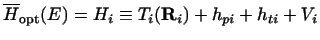
If there are more than 1 channel ( ), then
the same optical model Hamiltonian may be written with different
partitioning of the kinetic and internal energies that are appropriate
for the different mass partitions. Thus,
there will be a way of writing the
optical channel Hamiltonian for each channel:
), then
the same optical model Hamiltonian may be written with different
partitioning of the kinetic and internal energies that are appropriate
for the different mass partitions. Thus,
there will be a way of writing the
optical channel Hamiltonian for each channel:
 |
|
|
(13) |
each with some effective potential Vi. This last term can always be separated into
diagonal and off-diagonal parts as
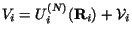 ,
where
,
where  is the term that couples together the
different channels. The separation is often made unique by requiring
that has zero diagonal matrix element.
The optical potentials (their sum labelled Vi in general) give rise to the elastic
scattering cross section, and the Optical Model procedure uses this causality in
reverse, to determine them as those local potentials which fit elastic scattering.
We typically look for optical potentials that vary only smoothly and slowly with
energy, as appropriate to averaging over some energy scale , and is most
often found just for the one channel case (N=1).
Note that in the coupled channels case (N>1) the diagonal potentials
is the term that couples together the
different channels. The separation is often made unique by requiring
that has zero diagonal matrix element.
The optical potentials (their sum labelled Vi in general) give rise to the elastic
scattering cross section, and the Optical Model procedure uses this causality in
reverse, to determine them as those local potentials which fit elastic scattering.
We typically look for optical potentials that vary only smoothly and slowly with
energy, as appropriate to averaging over some energy scale , and is most
often found just for the one channel case (N=1).
Note that in the coupled channels case (N>1) the diagonal potentials
 do not by themselves reproduce the elastic scattering without the work
of the off-diagonal couplings . We therefore call the diagonal
Ui(N) the bare potentials, because, even though they are
optical potentials which include the effects
of
do not by themselves reproduce the elastic scattering without the work
of the off-diagonal couplings . We therefore call the diagonal
Ui(N) the bare potentials, because, even though they are
optical potentials which include the effects
of  channels not in the model space, they do not include the dressing effects
of the inter-channel couplings within the model space .
Only the potential in the one-channel model space Ui(1)
is supposed to reproduce
the elastic scattering by itself.
Because
has Hermitian and anti-Hermitian parts,
the optical potentials will have real and imaginary terms, and because
is positive definite the imaginary parts will be negative
and absorptive.
channels not in the model space, they do not include the dressing effects
of the inter-channel couplings within the model space .
Only the potential in the one-channel model space Ui(1)
is supposed to reproduce
the elastic scattering by itself.
Because
has Hermitian and anti-Hermitian parts,
the optical potentials will have real and imaginary terms, and because
is positive definite the imaginary parts will be negative
and absorptive.
Next: 3 Model Schrödinger Equation
Up: Methods of Direct Reaction
Previous: 1 Direct Reaction Model
Prof Ian Thompson
2006-02-08