


Next: 3.1.0.1 Example 1 :
Up: 3 Basic theory and
Previous: 3 Basic theory and
The simplest calculation that can be performed with FRESCO is the
standard OM calculation. Here, the interaction between the projectile
and target is described in terms of a complex potential, whose imaginary
part accounts for the loss of flux in the elastic channel going to
any other channels.
The elastic differential cross section is evaluated through the expression1
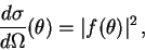 |
(1) |
where  is the scattering amplitude. The quantity
 represents the flux of particles elastically scattered by the target
at angle
represents the flux of particles elastically scattered by the target
at angle  , with v the asymptotic velocity of the outgoing
particles. This is obtained from the asymptotic expression of the
scattering wave function:
, with v the asymptotic velocity of the outgoing
particles. This is obtained from the asymptotic expression of the
scattering wave function:
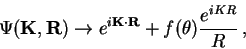 |
(2) |
where K denotes the incident linear momentum of the projectile
in the center of mass system and R is the relative coordinate
between projectile and target.
This in turn is calculated by solving the Schrödinger equation
for the complex potential U(R):
![\begin{displaymath}
\left[\frac{\hbar^{2}}{2\mu}\nabla^{2}+U(R)-E\right]\Psi(\mathbf{K},\mathbf{R})=0
\end{displaymath}](img10.png) |
(3) |
where  is the reduced mass and E is the energy in the center
of mass system:
is the reduced mass and E is the energy in the center
of mass system:
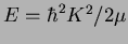 . This equation has a solution
with the form of a plane wave with relative momentum K
plus outgoing scattered waves:
. This equation has a solution
with the form of a plane wave with relative momentum K
plus outgoing scattered waves:
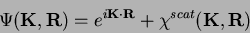 |
(4) |
where
 represents the set of scattered
waves. Notice that in absence of the target (U(R)=0) there are
not such scattered waves and
represents the set of scattered
waves. Notice that in absence of the target (U(R)=0) there are
not such scattered waves and
 .
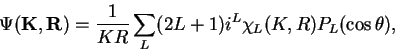
Commonly, the wave function
.
Commonly, the wave function
 is decomposed in partial
waves, in order to separate the angular and radial parts:
is decomposed in partial
waves, in order to separate the angular and radial parts:
 |
(5) |
where L is the orbital angular momentum between the projectile
and target and is the angle between K and R.
Replacing this solution into the Schrödinger equation (3)
we get the following equation for the radial functions 
![\begin{displaymath}
\left[\frac{\hbar^{2}}{2\mu}\frac{d^{2}}{dR^{2}}-\frac{\hbar^{2}}{2\mu}\frac{L(L+1)}{R^{2}}-U(R)+E\right]\chi_{L}(K,R)=0.
\end{displaymath}](img19.png) |
(6) |
Asymptotically, the radial functions behave as
Here, we distinguish two cases:
- U(R) is a purely short range potential (i.e., decays faster than
1/R). In this case
 ,
where hL(+) is a spherical Hankel function of the first kind
[1]
,
where hL(+) is a spherical Hankel function of the first kind
[1]
- U(R) contains a long range part. In this case,
 are
the so called Coulomb wave functions.
are
the so called Coulomb wave functions.
The coefficients SL are the scattering matrix (or S-matrix)
elements. They are related to the nuclear phase-shifts,  ,
by:
,
by:
 |
(7) |
These are very important quantities as all the information of the
effect that the target produces on the scattering wave function (and
hence in the observables) is contained in these coefficients. Hence
it is possible to write the all the scattering observables in terms
of the S-matrix elements. Notice that in the absence of target
SL=1 for all partial waves. Even in the presence of a point
Coulomb interaction, these coefficients remains equal to one, as the
Coulomb phase-shifts are already included in the Coulomb wave functions
HL(KR). It is also important to note that, if only real potentials
are involved, the S-matrices verify |SL|=1 and the phase
shifts are real numbers. This expresses the conservation
of flux of particles (i.e., the number of scattered particles equals
the number of incident particles). On the contrary, if the scattering
potential contains an imaginary part, then |SL|<1 and
become complex numbers. In this case, the outgoing flux of particles
is less than the incoming flux, indicating that part of the incident
flux leaves the elastic channel and goes to other channels.
Then, the calculation of the elastic cross section involves the following
steps:
- Integration of the differential equation (6) for
each value of L. The integration is carried out starting from R=0
and solving the differential equation in steps of
 up to
a certain maximum value Rm.
up to
a certain maximum value Rm.
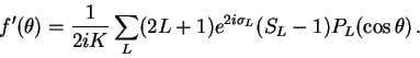
- For R large enough, the solution (5) obeys the asymptotic
form (2). Thus, choosing the value of Rm large
enough it is possible to identify the scattering amplitude
 )
comparison of (2) and the solution (5) for
R=Rm.
)
comparison of (2) and the solution (5) for
R=Rm.
 |
(8) |
- Finally, the differential elastic cross section is evaluated according
to Eq. (1).
It results obvious that the particular choice of and Rm
depends on each particular problem. If only short-ranged potentials
are involved (eg. neutron scattering) the value of Rm should
be chosen outside of the range of the projectile-target interaction.
However, in general U(R) has both Coulomb and nuclear parts. The
Coulomb part has a long (``infinite'') range that requires special
treatment. Actually, in this case the asymptotic solution of (3)
does not behave as planes waves and so expression (2)
is not strictly valid. In particular, planes waves should be replaced
by the so called Coulomb functions, which are the solutions of the
Schrodinger equation in presence of the Coulomb potential alone. For
our purposes, the important point to remind is that in that when long-range
interactions are present, the radial equations have to be solved up
to larger distances in order to ``reach'' their asymptotic form.
Concerning the radial step, , its choice will depend mainly
on the diffusiveness of the potentials. Very abrupt or sharp potentials
will normally require an smaller step.
Finally, a maximum value of L, denoted (Lmax) has to be chosen.
In principle, the sum in (5) goes to infinity. In practice,
convergence of the scattering observables is achieved for finite values
of Lmax. Within a semiclassical picture, the orbital angular
momentum can be related to the impact parameter, b, and the incident
linear momentum by
 . This means that, for a fixed
incident energy, large impact parameters correspond also to large
values of the orbital angular momentum. If only short-ranged potentials
are present, these values of L do not feel the potential of the
target. In presence of the Coulomb potential, these large L values
are commonly identified with trajectories that explore uniquely the
Coulomb part of the projectile-target interaction.
. This means that, for a fixed
incident energy, large impact parameters correspond also to large
values of the orbital angular momentum. If only short-ranged potentials
are present, these values of L do not feel the potential of the
target. In presence of the Coulomb potential, these large L values
are commonly identified with trajectories that explore uniquely the
Coulomb part of the projectile-target interaction.
The parameters discussed above are controlled by the following variables
in fresco:
- -
- rmatch: Matching radius (Rm in the discussion above)
- -
- hcm: Radial step
- -
- lmax: Maximum partial wave. Fresco also allows fixing
the minimum partial wave, through the variable LMIN. However, in normal
calculations this will be set to zero.
In the pure optical model approach only the ground state of the projectile
and targets are considered explicitly. Thus, a OM calculation only
provides the elastic scattering cross section. The loss of flux effect
from the elastic channel to the excluded channels (excitations, rearrangement
reactions, etc) is assumed to be included in the imaginary part of
the optical potential.
Subsections
Next: 3.1.0.1 Example 1 :
Up: 3 Basic theory and
Previous: 3 Basic theory and
Antonio Moro
2004-10-27