Let consider the transfer reaction
| (37) |
When the coupling to intermediate channels is weak, it is reasonable
to evaluate the transition amplitude in Born Approximation (BA). In
the case of rearrangement reactions there are several ways to describe
the interaction between the different fragments, one for each partition.
For example, if we choose to describe the scattering in terms of the
nuclei of the entrance partition, the projectile target interaction
will be written as
| VAb=Vvb+Uab | (38) |
The interaction Vvb is the the potential which binds the v
valence particle to the b core. In general, it will be described
as a real potential (for which we use the notation V). The potential
Uab is the optical potential describing the scattering between
b and v. It will typically contain both real and imaginary parts
(we use the letter U). In this representation, known as prior form,
the transition amplitude for the transfer process is given by
Analogously, for the exit channel:
VaB=Vav+Uab. In this
case, the expression (39) reduces to:
In either prior and post form the differential cross section is calculated as:
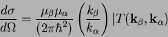 |
(42) |
According the previous expressions a basic ingredient required to
calculate the transfer amplitude in the prior DWBA approximation is
are the internal wave functions for the initial (
![]() )
and final (
)
and final (
![]() ) nuclei. In this scheme, the valence
particle v is bound to the b core to give the composite B.
In the simplest picture, the valence particle particle can be considered
a pure single-particle state. This means that, within in this extreme
model, there is only one possible configuration of the core and the
valence particle to give the nucleus B and thus, the wave function
for this nucleus can be written as:
) nuclei. In this scheme, the valence
particle v is bound to the b core to give the composite B.
In the simplest picture, the valence particle particle can be considered
a pure single-particle state. This means that, within in this extreme
model, there is only one possible configuration of the core and the
valence particle to give the nucleus B and thus, the wave function
for this nucleus can be written as:
| (43) |
In a more realistic model, however, the state of the composite contains
components of many single-particle states coupled to all possible
core states and thus, the wave function
![]() is built as a superposition of the form:
is built as a superposition of the form:
Example: the ground state of the 209Bi nucleus can modeled to a good approximation as a valence proton coupled to the core 208Pb. Due to the double close shell nature of the core, the valence proton can be regarded as a nearly pure single-particle state, occupying the 1h9/2 orbital. Then, we have: I=0, J=9/2,Notice that the integraland
. Moreover, as there is only one particle with this configuration, nB=1 in this case.
The bound wave functions
![]() obey the Schrodinger
equation3:
obey the Schrodinger
equation3:
| (46) |
The information required by FRESCO to construct the wave functions is provided in the section of form factors, which corresponds to the namelist &overlap/ in the fortran 90 version. However, the cfp's and the valence-target and core-target potentials are given in the couplings section, through the &coupling/ namelist.
It is important to note that the calculation of the transition amplitude
involves the integration in the channel coordinates
![]() and
and
![]() (see Fig. 3), which, after the
integration on the angular coordinates, becomes a integral in
(see Fig. 3), which, after the
integration on the angular coordinates, becomes a integral in ![]() and
and ![]() . Then, the coupled channels equations becomes:
. Then, the coupled channels equations becomes:
The integrals
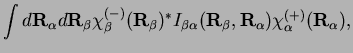
![\begin{displaymath}
\phi_{B}^{JM}(\xi,\mathbf{r})=\frac{1}{\sqrt{n_{B}}}\sum_{I\...
..._{b}^{I}(\xi)\otimes\varphi_{\ell sj}(\mathbf{r})\right]_{JM},
\end{displaymath}](img162.png)
![\includegraphics[%%
width=0.50\textwidth]{dwba/transfer.eps}](img189.png)