4 Fitting data: SFRESCO

A first calculation of cross sections using FRESCO will rarely be near the experimental data. Perhaps the reaction model is too simplified, or perhaps the input parameters are not accurate enough. The optical potential, binding potentials, spectroscopic amplitudes or R-matrix reduced widths could well be adjusted to see if the agreement between theory and experiment can be improved. The program SFRESCO searches for a $\chi^2$ minimum when comparing the outputs of FRESCO with sets of data, using the MINUIT search routines.

The inputs for SFRESCO specify the FRESCO input and output files, the number and types of search variables, and the experimental data sets to be compared with. These experimental data can be (type=0) an angular distribution for fixed energy, (1) an excitation and angular cross-section double distributions, or (2) an excitation cross section for fixed angle. They could also be (3) an excitation function for the total, reaction, fusion or inelastic cross section, (4) an excitation phase shift for fixed partial wave, (5) a desired factor for bound-state search, or (6) even a specific experimental constraint on some search parameter.

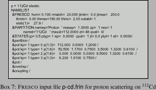
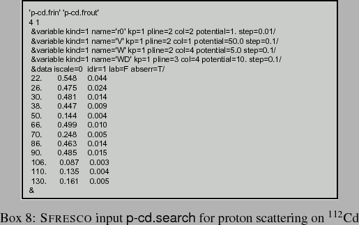
The simplest and most common fitting requirement is to determine an optical potential to fit the observed elastic scattering angular distribution. For example, to find a proton optical potential to fit cross sections for scattering on ¹¹²Cd at 27.90 MeV, we start with the normal FRESCO input of Box 7. The cross sections will be calculated at the experimental angles, not those specified here. In order to vary the real and imaginary potential strengths in this input, as well as the real radius, we have the search file for SFRESCO of Box 8. This search file begins by identifying the previous FRESCO input and naming the temporary output file, then giving the number of search variables and the number of experimental data sets.

Figure 6: Initial and fitted proton scattering on ¹¹²Cd at 27.9 MeV.

There are 3 &pot namelist lines in Box 7 for the nuclear parts of potential kp=1, so the variables of the interaction potentials (kind=1) in the search are identified by the specification of kp and pline in the &variable namelist in Box 8, along with col for the index to the p array. The potential value gives the initial value for the search, and step the initial magnitude for trial changes. Deformations can as well be searched upon. There are also parameters valmin and valmax,¹⁰to limit the range of that variable. Spectroscopic amplitudes to be varied (kind=2) are identified by the order nfrac in which they appear in the FRESCO input in a &cfp namelist, and then by their initial value afrac. Other variable kinds are described in the FRESCO input manual.

Experimental data sets are identified by their type specifications as listed above, and then by data_file for name of data file with data, which can be `=' for this search file, `<' for stdin (the default is `='). Then points gives the number of data points (default: keep reading as many as possible), lab is T or F for laboratory angles and cross sections (default false), and energy is lab energy for a type=0 dataset (default: use elab(1) from &fresco namelist). The abserr is true for absolute errors (default: false). Next, idir is -1 for cross-section data given as astrophysical S-factors, 0 for data given in absolute units (the default), and 1 as ratio to Rutherford. Finally, iscale is -1 for dimensionless data, and 0 absolute data in units of fm²/sr, 1 for b/sr, 2 for mb/sr (the default) and 3 for $\mu$b/sr.

With these two files (Boxes 7 and 8), SFRESCO is invoked interactively. First the name of the search file in Box 8 is given, then commands as in Table 2. A minimum set of commands will be p-cd.search / min / migrad / end / plot. The output plot file (default name search.plot) also contains the final values of the searched variables. The fitted parameters in this example are V=52.53 MeV, r0=1.179 fm, W=3.46 MeV and WD =7.43 MeV with ${\cal X}^2/N = 2.19$. The initial and final fits to the data are shown in Fig. 6.

Table 2: SFRESCO input commands. Words in typewriter font are to be replaced with user values.

Command	Operation
Q	query status of search variables
SET var val	set variable number var to value val.
FIX var	fix variable number var (set step=0).
STEP var step	unfix variable var with step step.
SCAN var val1 val2 step	scan variable var from value val1 to val2 in steps of step.
SHOW	list all datasets with current predictions and $\chi$ values.
LINE plotfile	write file (default: search.plot) with theoretical curves only.
READ file	read plot output file for further searches, if not:
READ snapfile	if the name of snapfile contains the string `snap',
	read last set of snap output snapfile from a previous fort.105.
ESCAN emin emax estep	scan lab. energy in incident channel
MIN	call MINUIT interactively.
MIGRAD	in MINUIT, perform MIGRAD search.
END	return to SFRESCO from MINUIT.
PLOT plotfile	write file (default: search.plot) with data and theory curves.
EX	exit (also at end of input file)